Imaging the following highly simplified broker-client market: at each time step, a client ask the broker for quotes; the broker provides a two-way quote — a bid price and an ask price for which the broker is willing to buy and sell respectively; the client can then choose to accept or reject.
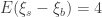
To model the client, we assume a client is either a buyer or seller (excluding hedge funds that could flip between buy and sell after seeing the quote). Each time step, only a unit number of security could be transacted. Each buyer or seller has an opinion on the true price of the security. We can use two random variables 


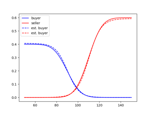
At the price where the blue and red cdfs intercept, it is the true mid price where

This true mid 
It is also advantageous for the broker to quote this true mid for his own benefit as on average, the buy and sell flows will match. Otherwise, the broker’s inventory will grow linearly with time. In this idealized model, there are two challenges for being the broker:
a) How does the broker know the true mid?
Broker is not running a grand auction which gives him a full picture on the distrubitions of
b) How to keep inventory size down?
Even if the broker knows the true mid and therefore on average the buy and sell flows cancel, the random nature of the orders make the fluctuation–or standard deviation–of the inventory size grow proportional to the square root of time. To keep inventory size under a limit, the broker has to skew the mid. For example, skew the mid below the true mid so it is more likely for a buyer to accept to get rid of a positive inventory. However, as on average the security is transacted at the true mid, the broker will lose some money due to the skew. He will have to charge some bid-ask to compensate the skew.
Optimal strategy for the broker
We can come up with an optimal strategy for the broker by breaking the problem into two parts according to the two questions above. The first problem is an online measurement problem. The second is a stochastic optimal control problem. As a first attempt, we do not try to optimize the bid-ask spread but assume the broker charge a small fixed bid-ask spread. Optimizing the bid-ask spread has to take into consideration the competition with other brokers for market share, which is not captured in this model anyway.
a) Online measurement
The true mid 
where 


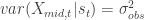
but the expectation of variance increases with time


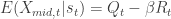
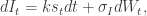
At time step t, after making a quote with mid price 


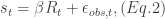
where 

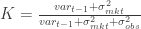
These can be used to update our estimate for mid at time t. In practice, the parameters 


where 
is the Kalman gain. Essentially, Eq. (1) is the state-transition model and Eq. (2) is the observation model. We use a Kalman filter to update our estimate for mid price online.
b) Stochastic optimal control
To make the problem analytically solvable, we approximate the our discrete model with a continuous one.
where 


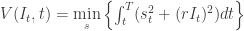
Suppose the cost function to optimize is
As the rate of accumulating inventory is linearly proportional to skew and the amount of money paid to offload the accumulated inventory is also proportional to skew, the 

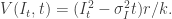
Using Hamilton–Jacobi–Bellman equation, we get the optimal control
and the associated cost function
The results mean we simply skew the quote proportional to the size of the inventory. Under this optimal control, the cost is accumulating at a speed of 

Simulation results
We can simulate the client behavior and the broker’s strategy as described above. In this simulation, the buyer and sellers have equal population. The standard deviations for 
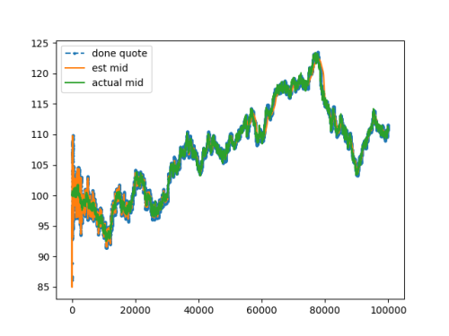
Inventory and PnL the broker makes are shown below. The inventory is usually below 10. During the time near t~8e4 when there is a stochastic trend going down, the inventory shoots to ~40, which also reflects as a drawdown in the PnL. The bid-ask spread is fixed at 0.75, at which the broker consistently makes a profit.


A zoom-in look at the quote below (Fig. 4 and 5) shows that the quote (estimated mid plus skew) actually tracks the true mid much better than the estimated mid. This is probably because in Eq. 2,
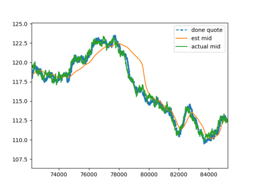
Fig. 4: Zoom-in of Fig. 2.
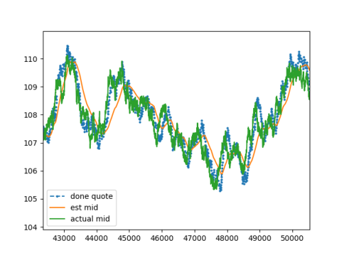
Fig. 5: Zoom-in of Fig. 2.

Leave a comment